Education Impact Analysis using ANOVA
REPORT ON:
Submitted by TEAM 09:
Jainam Shah
Singala Sri Sai
Sapa Bal Narendra
Sanvelly Vamshi Kanth Reddy
Under the guidance of:
Minkyu Kim (Adjunct Faculty)
ABSTRACT
Background:
We are given a dataset which has records of people with different levels of education i.e. Less than high school, High School, Jr College, Bachelor's, and Graduate along with the scores regarding their performance. Hence, people in the dataset are categorized into 5 different groups based on their level of education.
Purpose:
We want to identify whether the scores of people belonging to different levels of education are same or not. We can also phrase the question as is there any significant relevance of education on a person's score? If we were to pick people randomly from the given dataset for each group, is there a difference among their scores? If yes, is it due to some significant reasons (level of education) or due to randomness?
Methods:
We conducted analysis using ANOVA to compare the means of each group. As the number of groups are more than 2, we cannot use the T-Test or the Z-Test, as it would require n(n-1)/2 number of pariwise tests, increasing type-1 error rate. We first performed Exploratory Data Analysis (EDA) to prepare the dataset for anova and confirmed the intuitive assumptions regarding the data. We then formulated the hypothesis for ANOVA where the null hypothesis was that there is no difference among the means of the groups and the alterante hypothesis was atleast 1 group has different mean.
Results:
Based on our analysis, as the p-value was less than significance level and also the F-Statistic was greater than the F-Critical value, we rejected the null hypothesis in favour of the alternate hypothesis.
Conclusion:
With significant evidence, we can conclude that there is indeed difference among the means of groups (based on level of education) and that it is not due to randomness. Out of the 5 given groups, we found the following 2 pairs of groups to have different means: 1) "Less than high school" - "Graduate" and 2) "Less than high school" - "Bachelor's". Hence, we can say that people who have completed their Graduation or Bachelor's have different score than those who did not pass high school.
THEORY
What is ANOVA?
ANOVA (Analysis of Variance) is a statistical analysis technique that divides systematic components from random factors to account for the observed aggregate variability within a data set. The presented data set is statistically affected by the systematic factors but not by the random ones. The ANOVA test is used by analyst to evaluate the impact of independent factors on the dependent variables in a regression analysis. ANOVA is also called as Fisher Analysis of variance and it is the extension of the t-test and z-test.
Types of ANOVA:
- One-way ANOVA
- Two-way ANOVA
- N-way ANOVA
ANOVA Assumptions:
- Normally distributed population derives different group samples.
- The sample or distribution has a homogenous variance
- Analyst draw all the data in a sample independently.
ANOVA Formula:
ANOVA coefficient (F) = Mean sum of squares between the groups / Mean squares of Errors.
$ F = \frac{MSG}{MSE} $
INTERPRETATIONS:
The following is how the analyst can interpret the outcomes of the ANOVA test. The P-value is the ANOVA test’s most significant value. ANOVA test uses null hypothesis and alternative hypothesis. According to null hypothesis H0, all group means are equal and alternative hypothesis indicates that all the group means are not equal. When the p-value is less than 0.05 (or the specified significance level) analyst will reject the null hypothesis. Null hypothesis is accepted when the p-value is greater than 0.05 (or the specified significance level). Group means are not equal when analyst reject the null hypothesis
EXPLORATORY DATA ANALYSIS
### Import required libraries
import math
import numpy as np
import pandas as pd
import seaborn as sns
from scipy import stats
from sqlite3 import connect
import matplotlib.pyplot as plt

# Ignore Warnings
import warnings
warnings.filterwarnings('ignore')

### Required constants
DB_PATH = "../../dataset/dataset.db"
TABLE_NAME = "prj1"
<frozen importlib._bootstrap>:228: RuntimeWarning: scipy._lib.messagestream.MessageStream size changed, may indicate binary incompatibility. Expected 56 from C header, got 64 from PyObject
Read the database from .db file
### Connect to sqlite3 database
connection = connect(DB_PATH)

### Create pandas dataframe for analysis
query = "SELECT * FROM " + TABLE_NAME
df = pd.read_sql(query, connection)
print(df)
      index  Less than HS    45
0         0  Less than HS  26.0
1         1  Less than HS  43.8
2         2  Less than HS  34.4
3         3  Less than HS  76.2
4         4  Less than HS   0.2
...     ...           ...   ...
1166   1166      Graduate  52.7
1167   1167      Graduate  59.8
1168   1168      Graduate  54.1
1169   1169      Graduate  39.9
1170   1170      Graduate  58.2

[1171 rows x 3 columns]
Metadata - Information regarding the columns of dataset
df.info()
<class 'pandas.core.frame.DataFrame'>
RangeIndex: 1171 entries, 0 to 1170
Data columns (total 3 columns):
 #   Column        Non-Null Count  Dtype
---  ------        --------------  -----
 0   index         1171 non-null   int64
 1   Less than HS  1171 non-null   object
 2   45            1160 non-null   float64
dtypes: float64(1), int64(1), object(1)
memory usage: 27.6+ KB
Modify column names / types
df.rename(columns = {"Less than HS": "Education Level", "45": "Score"}, inplace = True)
df.drop(columns = ["index"], inplace = True)
print(df.head())
  Education Level  Score
0    Less than HS   26.0
1    Less than HS   43.8
2    Less than HS   34.4
3    Less than HS   76.2
4    Less than HS    0.2
Basic stats about each numerical feature
print(df.describe())
             Score
count  1160.000000
mean     40.726724
std      15.166281
min       0.200000
25%      30.300000
50%      41.000000
75%      51.325000
max      86.400000
Unique values for the categorical featue
print("Following are the unique values corresponding to the feature 'Education Level' :")
for idx, edu_lvl in enumerate(df['Education Level'].unique()):
    print(str(idx + 1) + " " + edu_lvl)
Following are the unique values corresponding to the feature 'Education Level' :
1 Less than HS
2 HS
3 Jr Coll
4 Bachelor's
5 Graduate
Visualize unique values count
fig, ax = plt.subplots(figsize= (8, 6))

sns.countplot(df['Education Level'], ax = ax)
ax.set_ylabel("Count")
Text(0, 0.5, 'Count')

Handle null / missing values
### Null values for each category
print("Following are the null values corresponding to each value of 'Education Level' :")
for idx, edu_lvl in enumerate(df['Education Level'].unique()):
    print(str(idx + 1) + " " + edu_lvl + " " + str(df[df['Education Level'] == edu_lvl].isna().sum()[1]))

print("Total Null Values: ", df.isna().sum()[1])
Following are the null values corresponding to each value of 'Education Level' :
1 Less than HS 2
2 HS 5
3 Jr Coll 1
4 Bachelor's 1
5 Graduate 2
Total Null Values:  11
### Visualize each value's distribution
temp_frames = []
fig, ax = plt.subplots(figsize= (8, 6))

for idx, edu_lvl in enumerate(df['Education Level'].unique()):
    temp_frames.append(df[df['Education Level'] == edu_lvl].drop(columns = \
                                ['Education Level']).rename(columns = {"Score": edu_lvl}))

temp_df = pd.concat(temp_frames).reset_index(drop = True)
axis = sns.boxplot(x = "variable", y = "value", data = pd.melt(temp_df), ax = ax)
axis.set(xlabel = 'Education Level', ylabel = 'Score')
plt.show()
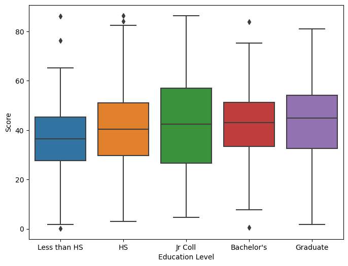
### Basic stats for each category in Education Level
print(temp_df.describe())
       Less than HS          HS    Jr Coll  Bachelor's    Graduate
count    118.000000  541.000000  96.000000  252.000000  153.000000
mean      36.528814   40.123105  41.004167   42.130556   43.612418
std       15.668517   14.886300  18.925799   13.480890   15.066123
min        0.200000    3.100000   4.700000    0.500000    1.800000
25%       27.600000   29.600000  26.525000   33.350000   32.600000
50%       36.400000   40.400000  42.450000   43.050000   44.800000
75%       45.300000   51.000000  57.025000   51.200000   54.200000
max       86.100000   86.300000  86.400000   83.900000   81.000000
### Mean value might not be an accurate measure for missing values due to outliers, so we are using median value
for frame in temp_frames:
    frame.fillna(frame.median(), inplace = True)

temp_df = pd.concat(temp_frames).reset_index(drop = True)
df = pd.melt(temp_df).dropna().reset_index(drop = True).rename(columns = \
                                                {"variable": "Education Level", "value": "Score"})
print(df)
     Education Level  Score
0       Less than HS   26.0
1       Less than HS   43.8
2       Less than HS   34.4
3       Less than HS   76.2
4       Less than HS    0.2
...              ...    ...
1166        Graduate   52.7
1167        Graduate   59.8
1168        Graduate   54.1
1169        Graduate   39.9
1170        Graduate   58.2

[1171 rows x 2 columns]
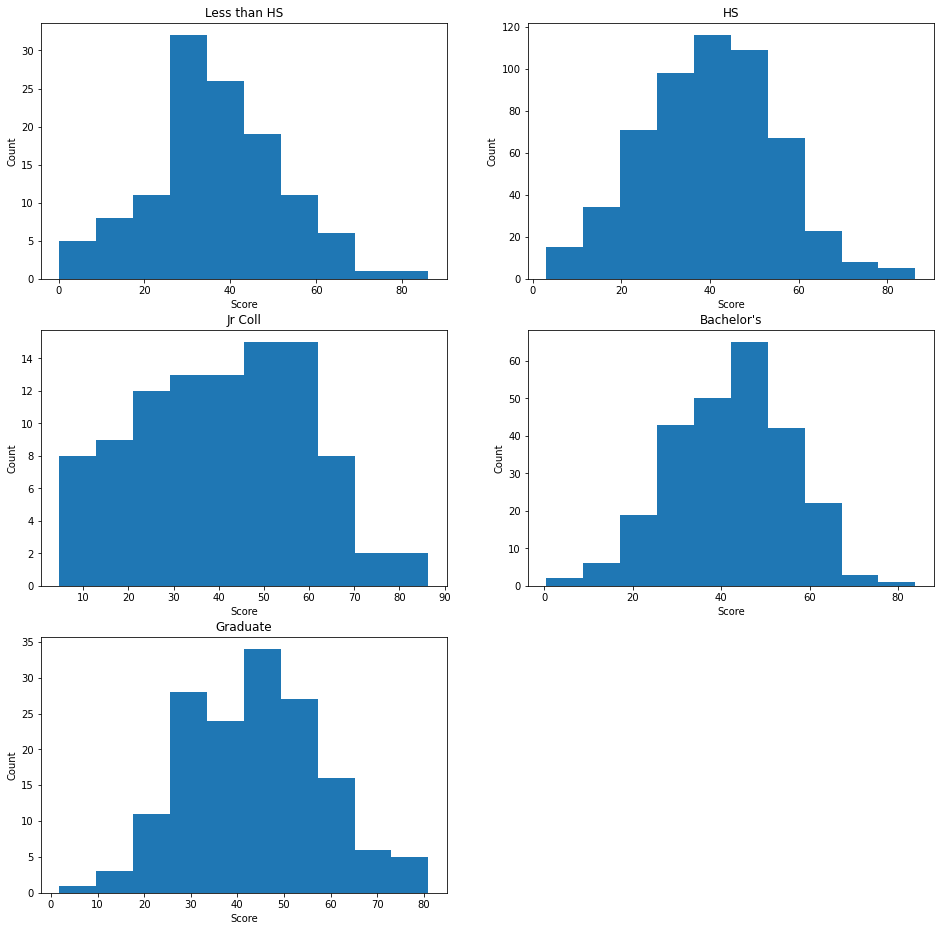
Visualize histogram of each category
### Matplot lib subplots
figure, axes = plt.subplots(3, 2, figsize=(16, 16))

# Less than HS
axes[0][0].hist(temp_frames[0])
axes[0][0].set_xlabel("Score")
axes[0][0].set_ylabel("Count")
axes[0][0].set_title("Less than HS")

# HS
axes[0][1].hist(temp_frames[1])
axes[0][1].set_xlabel("Score")
axes[0][1].set_ylabel("Count")
axes[0][1].set_title("HS")

# Jr Coll
axes[1][0].hist(temp_frames[2])
axes[1][0].set_xlabel("Score")
axes[1][0].set_ylabel("Count")
axes[1][0].set_title("Jr Coll")

# Bachelor's
axes[1][1].hist(temp_frames[3])
axes[1][1].set_xlabel("Score")
axes[1][1].set_ylabel("Count")
axes[1][1].set_title("Bachelor's")

# Graduate
axes[2][0].hist(temp_frames[4])
axes[2][0].set_xlabel("Score")
axes[2][0].set_ylabel("Count")
axes[2][0].set_title("Graduate")

figure.delaxes(axes[2][1])
plt.show()
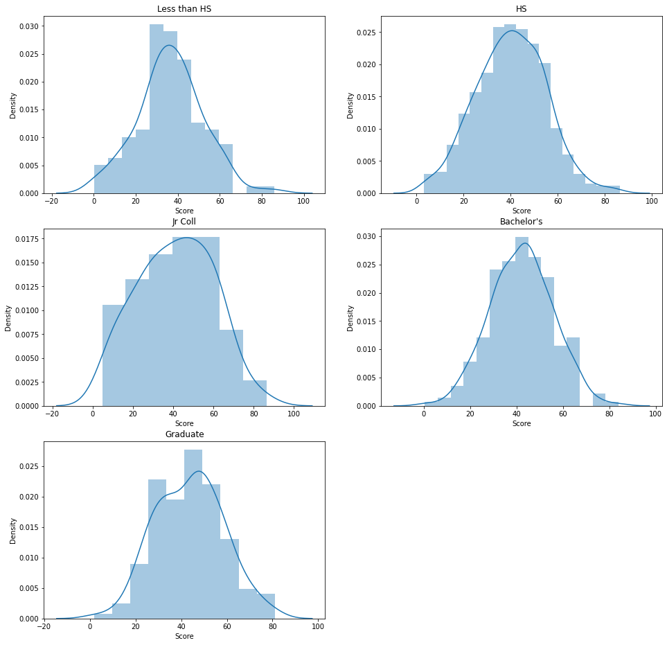
Density of each category using kde
figure, axes = plt.subplots(3, 2, figsize=(16, 16))

# Less than HS
sns.distplot(temp_frames[0], ax = axes[0][0])
axes[0][0].set_xlabel("Score")
axes[0][0].set_title("Less than HS")

# HS
sns.distplot(temp_frames[1], ax = axes[0][1])
axes[0][1].set_xlabel("Score")
axes[0][1].set_title("HS")

# Jr Coll
sns.distplot(temp_frames[2], ax = axes[1][0])
axes[1][0].set_xlabel("Score")
axes[1][0].set_title("Jr Coll")

# Bachelor's
sns.distplot(temp_frames[3], ax = axes[1][1])
axes[1][1].set_xlabel("Score")
axes[1][1].set_title("Bachelor's")

# Graduate
sns.distplot(temp_frames[4], ax = axes[2][0])
axes[2][0].set_xlabel("Score")
axes[2][0].set_title("Graduate")

figure.delaxes(axes[2][1])
plt.show()
ANOVA Analysis
**Defining hypothesis for testing:**
* Null Hypothesis
> $ H_0 $ = Means of all 5 groups are same, i.e. there is no significant difference among the means [ $ \mu_1 = \mu_2 = \mu_3 = \mu_4 = \mu_5 $ ]<br />
Alternative Hypothesis
$ H_A $ = Mean of atleast 1 group is different
If F-Statistic is greater than F-Critical value, we reject the null hypothesis.
### Degrees of Freedom
dfs = temp_frames
df_b = len(dfs) - 1 # For b/w groups = k - 1 where k is number of groups
df_w = len(df) - len(dfs) # For within groups = N - k where N is total samples from all groups and k is number of groups

### F-Critical Value
F_CR = stats.f.ppf(0.95, df_b, df_w) # Using alpha = 0.05 (significance level)
print("F-Critical Value: ", round(F_CR, 2))
F-Critical Value: 2.38
### Creating temp dataframes for each group
df_lhs = temp_df['Less than HS'].dropna()
df_hs = temp_df['HS'].dropna()
df_jrc = temp_df['Jr Coll'].dropna()
df_bs = temp_df["Bachelor's"].dropna()
df_gr = temp_df["Graduate"].dropna()
Calculating means for MSG and MSE
### Mean for each group and overall
mean_lhs = df_lhs.mean()
mean_hs = df_hs.mean()
mean_jrc = df_jrc.mean()
mean_bs = df_bs.mean()
mean_gr = df_gr.mean()
mean_overall = df["Score"].mean()

print("Mean for group 'Less than HS' \t:", round(mean_lhs, 2))
print("Mean for group 'HS' \t\t:", round(mean_hs, 2))
print("Mean for group 'Jr Coll' \t:", round(mean_jrc, 2))
print("Mean for group 'Less than HS' \t:", round(mean_bs, 2))
print("Mean for group 'Less than HS' \t:", round(mean_gr, 2))
print("Overall mean \t\t\t:", round(mean_overall, 2))
Mean for group 'Less than HS'   : 36.53
Mean for group 'HS'         : 40.13
Mean for group 'Jr Coll'    : 41.02
Mean for group 'Less than HS'   : 42.13
Mean for group 'Less than HS'   : 43.63
Overall mean            : 40.73
Calculating MSG and MSE for F-Statistic
### Util function for calculating sum_squred for each group
def sum_squared_within(series, mean):
    sum = 0
    for item in series:
        sum += (item - mean) ** 2
    return sum

def sum_squared_between(dfs, means, mean_overall):
    sum = 0
    for idx, _df in enumerate(dfs):
        sum += len(_df) * ((means[idx] - mean_overall) ** 2)
    return sum
dfs = [df_lhs, df_hs, df_jrc, df_bs, df_gr]
means = [mean_lhs, mean_hs, mean_jrc, mean_bs, mean_gr]

ss_lhs = sum_squared_within(df_lhs, mean_lhs)
ss_hs = sum_squared_within(df_hs, mean_hs)
ss_jrc = sum_squared_within(df_jrc, mean_jrc)
ss_bs = sum_squared_within(df_bs, mean_bs)
ss_gr = sum_squared_within(df_gr, mean_gr)

SSE = ss_lhs + ss_hs + ss_jrc + ss_bs + ss_gr
SSB = sum_squared_between(dfs, means, mean_overall)
SST = SSE + SSB
print("Sum Squared Between (SSB): ", round(SSB, 2))
print("Sum Squared Error (SSE): ", round(SSE, 2))
print("Sum Squared Total (SST): ", round(SST, 2))
Sum Squared Between (SSB):  4128.06
Sum Squared Error (SSE):  262540.11
Sum Squared Total (SST):  266668.17
### MSG and MSE
MSG = SSB / df_b
MSE = SSE / df_w
Calculating F-Statistic ($ F = \frac{MSG}{MSE} $) and p-value
F = MSG / MSE
p_val = stats.f.sf(F, df_b, df_w)
ANOVA Analysis Table
print ("\t\t\t sum_sq \t df \t\t F \t PR(>F)")
print("Between Groups \t\t " + str(round(SSB, 2)) + "\t" + str(df_b) + "\t\t" + \
      str(round(F, 2)) + "\t" + str(round(p_val, 5)))
print("Within Groups \t\t " + str(round(SSE, 2)) + "\t" + str(df_w) + "\t\t")
print("Total \t\t\t " + str(round(SST, 2)) + "\t" + str(df_w + df_b) + "\t\t")
             sum_sq      df          F   PR(>F)
Between Groups       4128.06    4       4.58    0.00112
Within Groups        262540.11  1166
Total            266668.17  1170
As the F-Statistic is greater than the F-Critical value (4.58 > 2.38), [also the p-value is less than alpha (0.00112 < 0.05)] we reject the null hypothesis. Hence, the mean of atleast one group is different.
To check which pairs of groups have different means, we need to perform multiple pairwise comparisons.
Pairwise Comparisons
### Creating a util function to perform t-test
def t_test(dfA, dfB, K, alpha = 0.05):
    h0 = 0 # Null Value
    SE = math.sqrt(((dfA.std() ** 2) / len(dfA)) + ((dfB.std() ** 2) / len(dfB))) # Standard Error
    T = abs(dfA.mean() - dfB.mean() - h0) / SE # T-Value =  diff - h0 / SE
    df = min(len(dfA) - 1, len(dfB) - 1) # Degrees of Freedom = min(n1-1, n2-1)
    p_val = stats.t.sf(T, df)
    rejectH0 = p_val < (alpha / K) # Bonferroni Correction:alpha* = alpha / K where K = k(k-1) / 2 and k = number of groups
    return (SE, T, df, p_val, rejectH0)
### Pairs for comparisons
pairs = [
    "BS:GR",
    "BS:HS",
    "BS:JRC",
    "BS:LHS",
    "GR:HS",
    "GR:JRC",
    "GR:LHS",
    "HS:JRC",
    "HS:LHS",
    "JRC:LHS"
]

pairs_df = {
    "BS": df_bs,
    "GR": df_gr,
    "HS": df_hs,
    "JRC": df_jrc,
    "LHS": df_lhs,
}

print("Group1:Group2 \t\t Std. Err. \t\t T \t\t  p-val \t alpha* \t  Reject H0")
K = (len(dfs) * (len(dfs) - 1)) / 2 # k*(k-1)/2 where k=number of groups-Bonferroni Correction for comparing multiple means

for pair in pairs:
    SE, T, _, p_val, rejectH0 = t_test(pairs_df[pair.split(":")[0]], pairs_df[pair.split(":")[1]], K)
    print(pair + "\t\t\t" + str(round(SE,4)) + "\t\t\t" + str(round(T, 4)) + "\t\t" + \
          str(round(p_val, 4)) + "\t\t" + str(0.05 / K) + "\t\t" + str(rejectH0))
Group1:Group2        Std. Err.       T        p-val      alpha*       Reject H0
BS:GR           1.47            1.016       0.1556      0.005       False
BS:HS           1.0572          1.8999      0.0293      0.005       False
BS:JRC          2.0904          0.5334      0.2975      0.005       False
BS:LHS          1.6513          3.3957      0.0005      0.005       True
GR:HS           1.3593          2.5764      0.0055      0.005       False
GR:JRC          2.2583          1.1551      0.1254      0.005       False
GR:LHS          1.8593          3.8192      0.0001      0.005       True
HS:JRC          2.0141          0.4436      0.3292      0.005       False
HS:LHS          1.5536          2.3166      0.0111      0.005       False
JRC:LHS         2.3803          1.8873      0.0311      0.005       False
Based on the pairwise comparisons, we can conclude that pairs of groups 1) "Bachelor's and Less than HS" and 2) "Graduate and Less than HS" have different means.
Confirming with homogenity tests
# Homogeneity using Bartlett & Levene Tests
w, pvalue = stats.bartlett(df['Score'][df['Education Level'] == 'Less than HS'],
                          df['Score'][df['Education Level'] == 'HS'],
                           df['Score'][df['Education Level'] == 'Jr Coll'],
                          df['Score'][df['Education Level'] == "Bachelor's"],
                          df['Score'][df['Education Level'] == 'Graduate'])

print("Bartlett's Test:\tw:{:7.4f}, pvalue:{:7.4f}".format(w, pvalue))

w, pvalue = stats.levene(temp_df['Less than HS'].dropna(), \
        temp_df['HS'].dropna(), temp_df['Jr Coll'].dropna(), temp_df["Bachelor's"].dropna(), temp_df['Graduate'].dropna())
print("Levene's Test:\t\tw:{:7.4f}, pvalue:{:7.4f}".format(w, pvalue))
Bartlett's Test:    w:17.5776, pvalue: 0.0015
Levene's Test:      w: 5.4545, pvalue: 0.0002
As the Bartlett's test and Levene's Test both have p-value < alpha* (0.005), we can conclude that our ANOVA analysis is true.
FINAL CONCLUSION
We reject the null hypothesis (means of all the groups are same), and there is indeed significant difference among the means of the groups. In layman terms, there is significant difference amonog the scores of individuals exposed to different levels of education.
To be more specific, people who completed their bachelors had significantly different score than those who did not passed high school. Those who completed their graduation also had significantly different score from those who did not passed high school. Based on multiple pairwise comparisons, we could not find significance difference among the rest of the pairs of groups.