Spam Classification using Logistic Regression
Spam Classification using Logistic Regression
Bal Narendra Sapa
Venkata Krishna Sreekar Padakandla
Sreeja Garlapati
Bharath Kondreddy
Sai Shara Vardhan Bandi
Instructor:
Minkyu Kim
ABSTRACT
Background:
We have a dataset that includes data on emails. Because we receive a large number of emails these days, email services have implemented spam detection to filter out unwanted messages. Logistic regression is one method that can be used to identify spam emails. This technique involves using certain characteristics of the emails to build a model that can classify them as spam or not spam
Purpose:
The goal of this project is to utilize various characteristics of the emails, such as the sender and recipient, to create a generalized linear model. We will then apply the logit function to this model to transform the output into probabilities. These probabilities, generated from the email attributes, will indicate whether the email is likely to be spam or not.
Methods:
We have been provided with 21 attributes. To begin, we have converted the categorical data into numerical data using one-hot encoding. We have then divided the dataset into a training set and a testing set in an 80/20 ratio. Using the stats.model library in Python, we have built a generalized linear model and linked it to the logit function. We have trained this model using the training dataset.
Results:
The model produces probabilities that show whether an email is spam or not. We use a threshold of 0.50 or 50% to classify emails. The model's accuracy ranges from 90% to 95%, depending on how the data is randomly divided. We also calculate precision, sensitivity, specificity, and other metrics to evaluate the model's performance.
Conclusion:
Our model, which was built using logistic regression and various attributes, is reliable. Based on its accuracy and other metrics, we can confidently say that it is effective at distinguishing spam emails from non-spam emails.
1. Business Understanding
The purpose of this project is to develop a spam filter that can identify the probability that an email is spam. We converted the characteristics into numerical data so that we could use logistic regression on it. The filter's ability to provide probabilities allows it to classify emails as spam or not spam. This spam filter enables the email software to offer spam filtering to its users, improving their satisfaction and increasing the number of users of the email service, leading to higher revenue.
2. Data Understanding
Before using the data to build a model, it is important to evaluate its quality and identify any missing or irrelevant information. In this case, there are two categorical attributes that need to be converted into numerical data in order to be used in the model. Once these attributes are converted, a threshold is determined based on the quality of the data. Additionally, there is a time attribute that needs to be converted into a format that can be used in the model using the datetime library. After conducting the logistic regression, the p-values for the coefficients in the table can be examined. If the p-value is greater than 0.05, it means that the coefficient does not significantly affect the probability value.
3. Data Preparation
Importing Libraries
import math
import numpy as np
import pandas as pd
import seaborn as sns
from sqlite3 import connect
import matplotlib.pyplot as plt
import statsmodels.api as sm
Retrieving the table from the SQLite database.
connection = connect("../../dataset/dataset.db")
query = "SELECT * FROM " + "prj2"
df = pd.read_sql(query, connection)
print(df.describe())
             index         spam  to_multiple         from           cc  \
count  3921.000000  3921.000000  3921.000000  3921.000000  3921.000000
mean   1960.000000     0.093599     0.158123     0.999235     0.404489
std    1132.039531     0.291307     0.364903     0.027654     2.666424
min       0.000000     0.000000     0.000000     0.000000     0.000000
25%     980.000000     0.000000     0.000000     1.000000     0.000000
50%    1960.000000     0.000000     0.000000     1.000000     0.000000
75%    2940.000000     0.000000     0.000000     1.000000     0.000000
max    3920.000000     1.000000     1.000000     1.000000    68.000000

        sent_email        image       attach       dollar      inherit  \
count  3921.000000  3921.000000  3921.000000  3921.000000  3921.000000
mean      0.277990     0.048457     0.132874     1.467228     0.038001
std       0.448066     0.450848     0.718518     5.022298     0.267899
min       0.000000     0.000000     0.000000     0.000000     0.000000
25%       0.000000     0.000000     0.000000     0.000000     0.000000
50%       0.000000     0.000000     0.000000     0.000000     0.000000
75%       1.000000     0.000000     0.000000     0.000000     0.000000
max       1.000000    20.000000    21.000000    64.000000     9.000000

            viagra     password     num_char  line_breaks       format  \
count  3921.000000  3921.000000  3921.000000  3921.000000  3921.000000
mean      0.002040     0.108136    10.706586   230.658505     0.695231
std       0.127759     0.959931    14.645786   319.304959     0.460368
min       0.000000     0.000000     0.001000     1.000000     0.000000
25%       0.000000     0.000000     1.459000    34.000000     0.000000
50%       0.000000     0.000000     5.856000   119.000000     1.000000
75%       0.000000     0.000000    14.084000   298.000000     1.000000
max       8.000000    28.000000   190.087000  4022.000000     1.000000

           re_subj  exclaim_subj  urgent_subj  exclaim_mess
count  3921.000000   3921.000000  3921.000000   3921.000000
mean      0.261413      0.080337     0.001785      6.584290
std       0.439460      0.271848     0.042220     51.479871
min       0.000000      0.000000     0.000000      0.000000
25%       0.000000      0.000000     0.000000      0.000000
50%       0.000000      0.000000     0.000000      1.000000
75%       1.000000      0.000000     0.000000      4.000000
max       1.000000      1.000000     1.000000   1236.000000
Transforming the time attribute into numerical data using the datetime library.
import datetime as dt
df['time'] = pd.to_datetime(df['time'])
df['time'] = df["time"].map(dt.datetime.toordinal)
df = df.query("number != 'none'")
Converting categorical data into numerical data using one-hot encoding.
df['winner'] = pd.get_dummies(df['winner'])['yes']
df['number'] = pd.get_dummies(df['number'])['big']
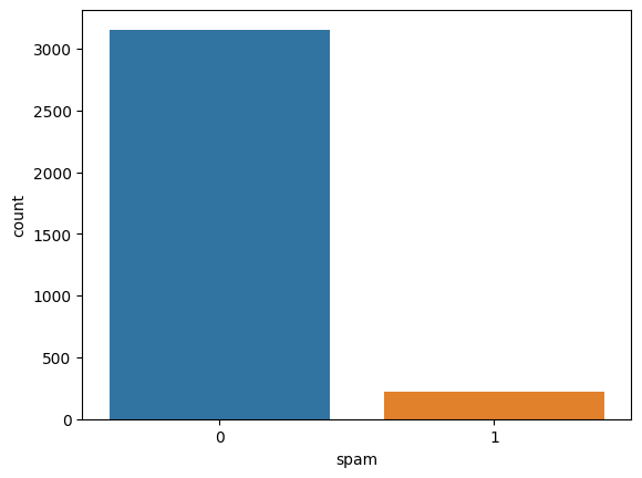
Exploratory Data Analysis
sns.countplot(df["spam"])
c:\Users\bnsap\anaconda3\lib\site-packages\seaborn\_decorators.py:36: FutureWarning: Pass the following variable as a keyword arg: x. From version 0.12, the only valid positional argument will be `data`, and passing other arguments without an explicit keyword will result in an error or misinterpretation.
  warnings.warn(


<Axes: xlabel='spam', ylabel='count'>
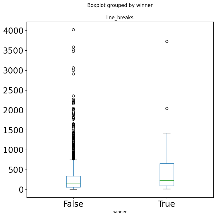
df.boxplot(column=['line_breaks'],by='winner',grid=False,figsize=(8,8),fontsize=20)
<Axes: title={'center': 'line_breaks'}, xlabel='winner'>
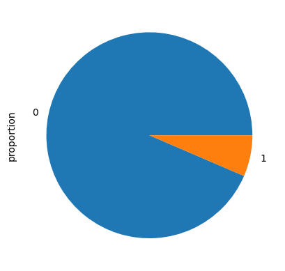
a= df["spam"].value_counts(normalize=True).plot.pie()
4. Logistic Regression Model
Dividing the dataset into a training set and a testing set.
test_data = df.sample(frac=0.2)
train_data = df.drop(test_data.index)

print(f"No. of training examples: {train_data.shape[0]}")
print(f"No. of testing examples: {test_data.shape[0]}")
No. of training examples: 2698
No. of testing examples: 674
Using the stats.model library to train the model.
Xtrain = train_data[['to_multiple', 'from', 'cc', 'sent_email', 'time',
       'image', 'attach', 'dollar', 'winner', 'inherit', 'viagra', 'password',
       'num_char', 'line_breaks', 'format', 're_subj', 'exclaim_subj',
       'urgent_subj', 'exclaim_mess', 'number']]
ytrain = train_data[['spam']]

log_reg = sm.GLM(ytrain.astype(float), Xtrain.astype(float), family = sm.families.Binomial(link = sm.families.links.logit())).fit()
Vanilla code for Logistic regression (without using any libraries)
Sigmoid function
def sigmoid(z):
    return 1 / (1 + np.exp(-z))
Prediction
def predict(X, w):
    z = np.dot(X, w[:-1,:]) + w[-1]
    probs = sigmoid(z)

    # Return the class with the highest probability
    return np.where(probs >= 0.5, 1, 0)
Learning of the model using the gradient descent (learning rate = 0.01)
def fit(X, y, learning_rate=0.01, num_iterations=10000):
    # Add a bias column to X
    X = np.c_[np.ones((X.shape[0], 1)), X]
    w = np.random.randn(X.shape[1], 1)

    for i in range(num_iterations):
        z = np.dot(X, w)
        probs = sigmoid(z)
        error = probs - y

        # Calculate the gradient of the error with respect to the weights
        gradient = np.dot(X.T, error)

        # Update the weights using the gradient and the learning rate
        w -= learning_rate * gradient

    return w
X = Xtrain.to_numpy()
y = ytrain.to_numpy()
w = fit(X, y)
predictions = predict(X, w)
C:\Users\bnsap\AppData\Local\Temp\ipykernel_11028\3196251242.py:2: RuntimeWarning: overflow encountered in exp
  return 1 / (1 + np.exp(-z))
Summary of model generated by stats.model
print(log_reg.summary())
                 Generalized Linear Model Regression Results
==============================================================================
Dep. Variable:                   spam   No. Observations:                 2698
Model:                            GLM   Df Residuals:                     2678
Model Family:                Binomial   Df Model:                           19
Link Function:                  logit   Scale:                          1.0000
Method:                          IRLS   Log-Likelihood:                -469.01
Date:                Thu, 14 Sep 2023   Deviance:                       938.02
Time:                        17:08:46   Pearson chi2:                 3.39e+03
No. Iterations:                    26   Pseudo R-squ. (CS):             0.1328
Covariance Type:            nonrobust
================================================================================
                   coef    std err          z      P>|z|      [0.025      0.975]
--------------------------------------------------------------------------------
to_multiple     -3.7024      0.729     -5.078      0.000      -5.132      -2.273
from          -925.7040   2326.983     -0.398      0.691   -5486.507    3635.099
cc              -0.0114      0.054     -0.211      0.833      -0.117       0.094
sent_email     -26.5907   1.55e+04     -0.002      0.999   -3.03e+04    3.03e+04
time             0.0013      0.003      0.397      0.691      -0.005       0.007
image           -1.8717      0.884     -2.118      0.034      -3.604      -0.140
attach           0.6756      0.227      2.982      0.003       0.232       1.120
dollar          -0.0728      0.035     -2.103      0.035      -0.141      -0.005
winner           2.1805      0.477      4.571      0.000       1.246       3.115
inherit          0.1931      0.177      1.093      0.275      -0.153       0.540
viagra           3.6670   7.34e+04      5e-05      1.000   -1.44e+05    1.44e+05
password        -0.4858      0.279     -1.738      0.082      -1.034       0.062
num_char        -0.0146      0.038     -0.383      0.701      -0.089       0.060
line_breaks     -0.0030      0.002     -1.652      0.098      -0.007       0.001
format          -0.7135      0.208     -3.431      0.001      -1.121      -0.306
re_subj         -2.0241      0.526     -3.846      0.000      -3.056      -0.993
exclaim_subj     0.1083      0.317      0.342      0.733      -0.513       0.729
urgent_subj      2.6611    4.1e+05   6.49e-06      1.000   -8.03e+05    8.03e+05
exclaim_mess     0.0123      0.002      5.069      0.000       0.008       0.017
number           0.8052      0.223      3.609      0.000       0.368       1.243
================================================================================
Examining the coefficients and how they influence the output.
Hypothesis testing for the coefficients: $$ H0 : \beta{coefficient} = 0 $$ $$ H1 : \beta{coefficient} \neq 0 $$
In hypothesis testing for the coefficients of the model, the null hypothesis is that the coefficient has no effect on the output (i.e., it is equal to zero), while the alternative hypothesis is that the coefficient does have an effect on the output (i.e., it is not equal to zero). If the p-value of a coefficient is greater than 0.05, it means that there is not enough evidence to reject the null hypothesis, and therefore it can be concluded that the coefficient does not have a significant effect on the output. In the summary table, some of the coefficients have p-values greater than 0.05, indicating that they do not have a significant effect on the output of the model.
Evaluating the model using the test dataset.
predictions using stats model
Xtest = test_data[['to_multiple', 'from', 'cc', 'sent_email', 'time',
       'image', 'attach', 'dollar', 'winner', 'inherit', 'viagra', 'password',
       'num_char', 'line_breaks', 'format', 're_subj', 'exclaim_subj',
       'urgent_subj', 'exclaim_mess', 'number']]
ytest = test_data['spam']

yhat = log_reg.predict(Xtest)
prediction = list(map(round, yhat))
predictions using vanilla code
predictions = predict(Xtest.to_numpy(), w)
C:\Users\bnsap\AppData\Local\Temp\ipykernel_11028\3196251242.py:2: RuntimeWarning: overflow encountered in exp
  return 1 / (1 + np.exp(-z))
5. Evaluation
1. Calculating the confusion matrix for stats model
cm = np.array([[0,0],[0,0]])
for i,j in zip(ytest, prediction):
    if i == j and i == 0:
        cm[0][0] = cm[0][0] + 1
    elif i == j and j == 1:
        cm[1][1] = cm[1][1] + 1
    elif i != j and i == 0:
        cm[0][1] = cm[0][1] + 1
    else:
        cm[1][0] = cm[1][0] + 1
cm
array([[625,   2],
       [ 40,   7]])
TP = cm[1][1]
TN = cm[0][0]
FP = cm[0][1]
FN = cm[1][0]
Accuracy
accuracy = (TP + TN)/(TP + TN + FP + FN)
accuracy
0.9376854599406528
Sensitivity
sensitivity = TP/(TP + FN)
sensitivity
0.14893617021276595
Specificity
specificity = TN/(TN + FP)
specificity
0.9968102073365231
Precision
Precision = TP/(TP + FP)
Precision
0.7777777777777778
2. Calculating the confusion matrix vanilla code
cm = np.array([[0,0],[0,0]])
for i,j in zip(predictions, ytest):
    if i == j and i == 0:
        cm[0][0] = cm[0][0] + 1
    elif i == j and j == 1:
        cm[1][1] = cm[1][1] + 1
    elif i != j and i == 0:
        cm[0][1] = cm[0][1] + 1
    else:
        cm[1][0] = cm[1][0] + 1
TP = cm[1][1]
TN = cm[0][0]
FP = cm[0][1]
FN = cm[1][0]
accuracy = (TP + TN)/(TP + TN + FP + FN)
cm
array([[627,  47],
       [  0,   0]])
accuracy
0.9243323442136498
Conclusion
In this model, a threshold of 0.5 or 50% is used to predict whether a given email is spam or not. The accuracy of the model is approximately 93%, which may vary slightly due to the random division of the dataset. This model has a specificity of 99.51%, meaning it is very accurate at correctly identifying negative examples (emails that are not spam). Based on these results, it can be concluded that the logistic regression model is effective at classifying whether a given email is spam or not.